摘要:
合集:AI案例-CV-传媒
数据集:手写数字图片MNIST数据集
数据集价值:常用于训练和测试机器学习算法
解决方案:PyTorch框架、全连接网络
一、问题描述
MNIST(Modified National Institute of Standards and Technology)手写数字数据集是一个广泛使用的数据库,常用于训练和测试机器学习算法,尤其是在计算机视觉和手写识别领域。许多关于神经网络的教程都会使用MNIST数据集作为例子来解释神经网络的工作原理。此外,许多研究者会使用MNIST数据集来比较和评估他们的算法和模型,并与其他研究者的结果进行比较。
数据集来源: MNIST数据集由美国国家标准与技术研究所(National Institute of Standards and Technology,NIST)发起整理,一共统计了来自250个不同的人手写数字图片。其中50%是高中生,50%来自人口普查局的工作人员。MNIST数据集是在20世纪90年代初期开始收集和整理的。最终在1994年正式发布,成为机器学习领域广泛使用的基准数据集之一。
二、数据集内容
关键信息
MNIST 数据集是计算机视觉领域中最重要的数据集之一,对于初学者和研究人员来说,它提供了一个相对简单但实用的平台来测试和训练机器学习模型。以下是关于MNIST数据集的一些关键信息:
数据集内容:MNIST 数据集包含手写数字的灰度图像,总共有10个类别(数字0到9)。
创建者:NIST
发布时间:1994年
图像大小:每张图像的尺寸是 28x28 像素。
数据集规模:训练集包含 60,000 张图像。测试集包含 10,000 张图像。
数据集特点:图像是标准化的,即它们被调整为固定大小,并且中心位于图像中心。图像是灰度的,即每个像素只有一个灰度值。
使用场景:由于其简单性和标准化,MNIST 数据集通常作为深度学习和机器学习入门教程的基准数据集。它被广泛用于训练和评估各种图像识别模型,包括卷积神经网络(CNN)。
深度学习框架支持:许多深度学习框架,如 TensorFlow、Keras、PyTorch 和 Caffe,都提供了内置的支持或易于使用的接口来加载和处理 MNIST 数据集。
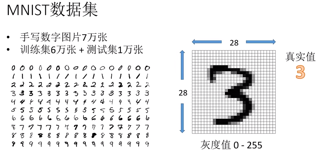
图:MNIST数据集内容
数据集使用许可协议
MIT
读取数据集样例
源码:read-mnist.py
import os.path
import gzip
import pickle
import os
import numpy as np
from PIL import Image
key_file = {
'train_img':'train-images-idx3-ubyte.gz',
'train_label':'train-labels-idx1-ubyte.gz',
'test_img':'t10k-images-idx3-ubyte.gz',
'test_label':'t10k-labels-idx1-ubyte.gz'
}
#dataset_dir = os.path.dirname(os.path.abspath(__file__))
dataset_dir = '.'
save_file = dataset_dir + "/mnist.pkl"
train_num = 60000
test_num = 10000
img_dim = (1, 28, 28)
img_size = 784
def _load_label(file_name):
file_path = dataset_dir + "/MNIST/raw/" + file_name
print("Converting " + file_name + " to NumPy Array ...")
with gzip.open(file_path, 'rb') as f:
labels = np.frombuffer(f.read(), np.uint8, offset=8)
print("Done")
return labels
def _load_img(file_name):
file_path = dataset_dir + "/MNIST/raw/" + file_name
print("Converting " + file_name + " to NumPy Array ...")
with gzip.open(file_path, 'rb') as f:
data = np.frombuffer(f.read(), np.uint8, offset=16)
data = data.reshape(-1, img_size)
print("Done")
return data
def _convert_numpy():
dataset = {}
dataset['train_img'] = _load_img(key_file['train_img'])
dataset['train_label'] = _load_label(key_file['train_label'])
dataset['test_img'] = _load_img(key_file['test_img'])
dataset['test_label'] = _load_label(key_file['test_label'])
return dataset
def init_mnist():
dataset = _convert_numpy()
print("Creating pickle file ...")
with open(save_file, 'wb') as f:
pickle.dump(dataset, f, -1)
print("Done!")
def _change_one_hot_label(X):
T = np.zeros((X.size, 10))
for idx, row in enumerate(T):
row[X[idx]] = 1
return T
def load_mnist(normalize=True, flatten=True, one_hot_label=False):
"""读入MNIST数据集
Parameters
----------
normalize : 将图像的像素值正规化为0.0~1.0
one_hot_label :
one_hot_label为True的情况下,标签作为one-hot数组返回
one-hot数组是指[0,0,1,0,0,0,0,0,0,0]这样的数组
flatten : 是否将图像展开为一维数组
Returns
-------
(训练图像, 训练标签), (测试图像, 测试标签)
"""
if not os.path.exists(save_file):
init_mnist()
with open(save_file, 'rb') as f:
dataset = pickle.load(f)
if normalize:
for key in ('train_img', 'test_img'):
dataset[key] = dataset[key].astype(np.float32)
dataset[key] /= 255.0
if one_hot_label:
dataset['train_label'] = _change_one_hot_label(dataset['train_label'])
dataset['test_label'] = _change_one_hot_label(dataset['test_label'])
if not flatten:
for key in ('train_img', 'test_img'):
dataset[key] = dataset[key].reshape(-1, 1, 28, 28)
return (dataset['train_img'], dataset['train_label']), (dataset['test_img'], dataset['test_label'])
def read_smaple_data():
# 第一次调用会花费几分钟 ……
(x_train, t_train), (x_test, t_test) = load_mnist(flatten=True,
normalize=False)
# 输出各个数据的形状
print(x_train.shape) # (60000, 784)
print(t_train.shape) # (60000,)
print(x_test.shape) # (10000, 784)
print(t_test.shape) # (10000,)
def show_sample_img():
(x_train, t_train), (x_test, t_test) = load_mnist(flatten=True, normalize=False)
img = x_train[10]
label = t_train[10]
print(label) # 5
print(img.shape) # (784,)
img = img.reshape(28, 28) # 把图像的形状变为原来的尺寸
print(img.shape) # (28, 28)
pil_img = Image.fromarray(np.uint8(img))
pil_img.show()
若调用read_smaple_data()函数,输出mnist.pkl序列化文件:
if __name__ == '__main__':
    read_smaple_data()
    # show_sample_img()
当没有mnist.pkl序列化二进制文件时候,在data-code目录下执行
python read-mnist.py
结果如下:
Converting train-images-idx3-ubyte.gz to NumPy Array ...
Done
Converting train-labels-idx1-ubyte.gz to NumPy Array ...
Done
Converting t10k-images-idx3-ubyte.gz to NumPy Array ...
Done
Converting t10k-labels-idx1-ubyte.gz to NumPy Array ...
Done
Creating pickle file: mnist.pkl ...
Done!
(60000, 784)
(60000,)
(10000, 784)
(10000,)
三、搭建神经网络
神经网络
神经网络是一种受人类大脑神经结构启发的计算模型,广泛应用于模式识别、分类、回归等任务中。它通过多层神经元的层级结构对数据进行逐层处理,从而从复杂的非线性数据中提取特征和模式。以下是关于神经网络的基本组成部分和工作原理的详细介绍:
基本组成部分
- 输入层:负责接收输入数据,每个节点(或神经元)对应一个输入特征。
- 隐藏层:位于输入层和输出层之间,是神经网络的核心部分,负责提取和转换特征。
- 输出层:根据具体任务输出最终结果,神经元数量和激活函数的选择取决于任务类型。
- 神经元:神经网络的基本计算单元,模拟了生物神经元的工作机制,通过加权求和和非线性激活函数处理后生成输出。
以下使用MNIST数据集搭建神经网络。神经网络的输入层有784个神经元,输出层有10个神经元。输入层的784这个数字来源于图像大小的28×28=784,输出层的10这个数字来源于10类别分类(数字0到9,共10类别)。此外,这个神经网络有2个隐藏层,第1个隐藏层有50个神经元,第2个隐藏层有100个神经元。这个隐藏层个数、50和100神经元个数可以设置为任何值。
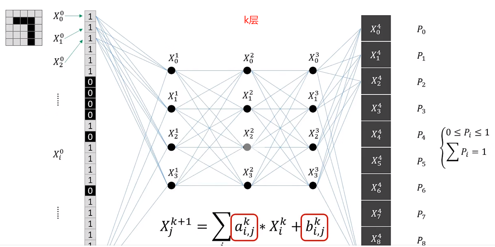
图:识别5*5图片的神经网络
神经网络中的a和b是网络参数;X(上标k,下标j)为第k层网络中第j个神经单元的权重,且每一层权重X的汇总值为1; P(i)代表图片识别后为i的概率,P(i)汇总值为1。
工作原理
神经网络的工作原理包括前向传播和反向传播两个过程。前向传播是指将输入信号通过网络向前传递,经过一系列的加权求和和激活函数操作,最终得到输出结果的过程。反向传播则是根据预测结果与真实值的误差,通过计算损失函数相对于每个权重的梯度,并沿着梯度的方向更新权重,以使损失函数最小化。神经网络训练的过程就是调整权重参数值。
激活函数
激活函数是神经网络的核心,它引入了非线性,使得网络可以处理复杂的非线性数据关系。常用的激活函数包括Sigmoid函数、Tanh函数和ReLU函数等。
应用领域
神经网络的应用领域非常广泛,包括图像识别、自然语言处理、推荐系统、金融预测、医疗诊断等。
神经网络通过模拟人脑的神经元网络结构,能够处理复杂的非线性问题,并在多个领域取得了显著的成果。随着技术的不断进步,神经网络的应用前景将更加广阔。
安装
参考《安装深度学习框架PyTorch》,安装CPU版或GPU版PyTorch框架。以下为简化版安装方法:
conda create -n pytorch-env python=3.10
conda activate pytorch-env
conda install numpy pytorch torchvision matplotlib
源码实现
源码:pytorch-mnist.py
1、加载开发包
import torch
from torch.utils.data import DataLoader
from torchvision import transforms
from torchvision.datasets import MNIST
import matplotlib.pyplot as plt
2、定义神经网络模型
以下代码这段代码使用PyTorch框架定义了一个简单的神经网络模型,该模型包含四个全连接层(也称为线性层),并使用 ReLU(Rectified Linear Unit)激活函数。ReLU函数定义为当输入大于或等于 0 时,函数值为输入本身;当输入小于 0 时,函数值为 0。
在 __init__ 方法中,我们定义了四个全连接层:
self.fc1:输入维度为 28 * 28(对应于 28×28 的图像),输出维度为 64。self.fc2:输入维度为 64,输出维度为 64。self.fc3:输入维度为 64,输出维度为 64。self.fc4:输入维度为 64,输出维度为 10(对应于 10 类分类任务)。
forward 方法定义了数据在网络中的前向传播过程:
- 输入
x首先通过self.fc1层,然后应用 ReLU 激活函数。 - 输出通过
self.fc2层,再次应用 ReLU 激活函数。 - 输出通过
self.fc3层,继续应用 ReLU 激活函数。 - 最后,输出通过
self.fc4层,并应用log_softmax函数。log_softmax函数将输出转换为对数概率分布,这在多分类任务中很常见。dim=1参数表示沿着第二个维度(即类别维度)进行 softmax 操作。softmax()用于将一组任意实数转换为表示概率分布的[0,1]之间的实数。它本质上是一种归一化函数。
class Net(torch.nn.Module):
    def __init__(self):
        super().__init__()
        self.fc1 = torch.nn.Linear(28*28, 64)
        self.fc2 = torch.nn.Linear(64, 64)
        self.fc3 = torch.nn.Linear(64, 64)
        self.fc4 = torch.nn.Linear(64, 10)

    def forward(self, x):
        x = torch.nn.functional.relu(self.fc1(x))
        x = torch.nn.functional.relu(self.fc2(x))
        x = torch.nn.functional.relu(self.fc3(x))
        x = torch.nn.functional.log_softmax(self.fc4(x), dim=1)
        return x
3、加载数据
def get_data_loader(is_train):
    to_tensor = transforms.Compose([transforms.ToTensor()])
    data_set = MNIST(root='.', train=is_train, transform=to_tensor, download=True)
    return DataLoader(data_set, batch_size=15, shuffle=True)
4、定义评估函数
这段代码定义了一个名为 evaluate 的函数,用于评估神经网络模型在测试数据集上的性能。
函数初始化两个计数器:
n_correct:用于记录模型预测正确的样本数量。n_total:用于记录测试数据集中的总样本数量。
使用 with torch.no_grad() 上下文管理器可以确保在评估过程中不计算梯度,从而节省计算资源。
对于测试数据集中的每个样本(x, y),执行以下操作:
- 将输入特征
x调整为模型所需的形状(在这里是[batch_size, 28 * 28],其中batch_size是批量大小)。 - 将调整后的输入特征传递给模型,并获取模型的输出
outputs。 - 对于每个输出
output,使用torch.argmax函数找到概率最高的类别索引,并将其与真实标签y[i]进行比较。如果它们相等,则将n_correct计数器加 1。 - 将
n_total计数器加 1,表示已处理一个样本。
返回准确率:return n_correct / n_total 计算并返回模型在测试数据集上的准确率,即预测正确的样本数量除以总样本数量。
def evaluate(test_data, net):
    n_correct = 0
    n_total = 0
    with torch.no_grad():
        for (x, y) in test_data:
            outputs = net.forward(x.view(-1, 28*28))
            for i, output in enumerate(outputs):
                if torch.argmax(output) == y[i]:
                    n_correct += 1
                n_total += 1
    return n_correct / n_total
5、模型训练
定义了一个名为 main 的函数。定义一个 Adam 优化器,用于优化模型的参数。学习率设置为 0.001。
训练过程包含两个 epoch(迭代次数),每个 epoch 都遍历训练数据集。对于每个样本(x, y),执行以下操作:
- 使用
net.zero_grad()清除之前的梯度。 - 将输入特征
x调整为模型所需的形状(在这里是[batch_size, 28 * 2GLU)。 - 将调整后的输入特征传递给模型,并获取模型的输出
output。 - 使用
torch.nn.functional.nll_loss函数计算损失(负对数似然损失)。 - 使用
loss.backward()计算梯度。 - 使用
optimizer.step()更新模型的参数。
在每个 epoch 结束时,评估模型在测试数据集上的准确率,并打印出来。
可视化预测结果:遍历测试数据集的前四个样本,并对每个样本执行以下操作:
- 使用
torch.argmax函数找到概率最高的类别索引。 - 使用
plt.imshow函数显示输入图像。 - 使用
plt.title函数显示预测结果。
最后,使用 plt.show() 显示所有图像。
def main():
train_data = get_data_loader(is_train=True)
test_data = get_data_loader(is_train=False)
net = Net()
print("initial accuracy:", evaluate(test_data, net))
optimizer = torch.optim.Adam(net.parameters(), lr=0.001)
for epoch in range(2):
for (x, y) in train_data:
net.zero_grad()
output = net.forward(x.view(-1, 28*28))
loss = torch.nn.functional.nll_loss(output, y)
loss.backward()
optimizer.step()
print("epoch", epoch, "accuracy:", evaluate(test_data, net))
for (n, (x, _)) in enumerate(test_data):
if n > 3:
break
predict = torch.argmax(net.forward(x[0].view(-1, 28*28)))
plt.figure(n)
plt.imshow(x[0].view(28, 28))
plt.title("prediction: " + str(int(predict)))
plt.show()
if __name__ == "__main__":
main()
6、推理运行结果
在data-code目录下执行:
python pytorch-mnist.py
Using downloaded and verified file: .\MNIST\raw\t10k-labels-idx1-ubyte.gz
Extracting .\MNIST\raw\t10k-labels-idx1-ubyte.gz to .\MNIST\raw
initial accuracy: 0.0982
epoch 0 accuracy: 0.9486
epoch 1 accuracy: 0.9669
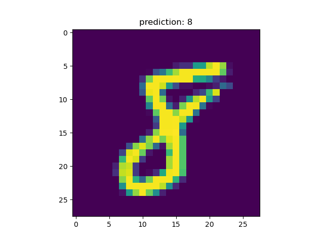
对于一手写字符为8的测试图片推理出分类8。
四、参考资料
源数据集数据结构
FILE FORMATS FOR THE MNIST DATABASE
The data is stored in a very simple file format designed for storing vectors and multidimensional matrices. General info on this format is given at the end of this page, but you don’t need to read that to use the data files.
All the integers in the files are stored in the MSB first (high endian) format used by most non-Intel processors. Users of Intel processors and other low-endian machines must flip the bytes of the header.
There are 4 files:“
train-images-idx3-ubyte: training set images`
train-labels-idx1-ubyte: training set labels
t10k-images-idx3-ubyte: test set images
t10k-labels-idx1-ubyte: test set labels
The training set contains 60000 examples, and the test set 10000 examples.
The first 5000 examples of the test set are taken from the original NIST training set. The last 5000 are taken from the original NIST test set. The first 5000 are cleaner and easier than the last 5000.
TRAINING SET LABEL FILE (train-labels-idx1-ubyte):
[offset] [type]     [value]     [description]`
`0000   32 bit integer 0x00000801(2049) magic number (MSB first)`
`0004   32 bit integer 60000      number of items`
`0008   unsigned byte  ??        label`
`0009   unsigned byte  ??        label`
`........`
`xxxx   unsigned byte  ??        label
The labels values are 0 to 9.
TRAINING SET IMAGE FILE (train-images-idx3-ubyte):
[offset] [type]     [value]     [description]`
`0000   32 bit integer 0x00000803(2051) magic number`
`0004   32 bit integer 60000      number of images`
`0008   32 bit integer 28        number of rows`
`0012   32 bit integer 28        number of columns`
`0016   unsigned byte  ??        pixel`
`0017   unsigned byte  ??        pixel`
`........`
`xxxx   unsigned byte  ??        pixel
Pixels are organized row-wise. Pixel values are 0 to 255. 0 means background (white), 255 means foreground (black).
TEST SET LABEL FILE (t10k-labels-idx1-ubyte):
[offset] [type]     [value]     [description]`
`0000   32 bit integer 0x00000801(2049) magic number (MSB first)`
`0004   32 bit integer 10000      number of items`
`0008   unsigned byte  ??        label`
`0009   unsigned byte  ??        label`
`........`
`xxxx   unsigned byte  ??        label
The labels values are 0 to 9.
TEST SET IMAGE FILE (t10k-images-idx3-ubyte):
[offset] [type]     [value]     [description]`
`0000   32 bit integer 0x00000803(2051) magic number`
`0004   32 bit integer 10000      number of images`
`0008   32 bit integer 28        number of rows`
`0012   32 bit integer 28        number of columns`
`0016   unsigned byte  ??        pixel`
`0017   unsigned byte  ??        pixel`
`........`
`xxxx   unsigned byte  ??        pixel
Pixels are organized row-wise. Pixel values are 0 to 255. 0 means background (white), 255 means foreground (black).
THE IDX FILE FORMAT
the IDX file format is a simple format for vectors and multidimensional matrices of various numerical types.
The basic format is
magic number`
`size in dimension 0`
`size in dimension 1`
`size in dimension 2`
`.....`
`size in dimension N`
`data
The magic number is an integer (MSB first). The first 2 bytes are always 0.
The third byte codes the type of the data: 0x08: unsigned byte 0x09: signed byte 0x0B: short (2 bytes) 0x0C: int (4 bytes) 0x0D: float (4 bytes) 0x0E: double (8 bytes)
The 4-th byte codes the number of dimensions of the vector/matrix: 1 for vectors, 2 for matrices….
The sizes in each dimension are 4-byte integers (MSB first, high endian, like in most non-Intel processors).
The data is stored like in a C array, i.e. the index in the last dimension changes the fastest.