FER2013人脸表情检测数据集和CNN检测模型

需要登录后才允许下载文件包。登录

合集：AI案例-CV-人类生理心理
数据集：FER2013(Facial Expression Recognition)数据集
AI问题：图像分类
数据集价值：统一的数据集为不同研究团队提供共同评估基准，方便比较不同算法和模型的性能，促进学术交流和技术进步。
解决方案：Tensorflow框架、CNN模型

一、问题描述

FER-2013(Facial Expression Recognition)数据集由Pierre-Luc Carrier和Aaron Courville创建。作为计算机视觉和人脸表情识别研究的一部分。FER-2013 数据集广泛用于训练和评估用于人脸表情识别的机器学习算法，尤其是卷积神经网络（CNN）等深度学习模型。

二、数据集内容

FER-2013 数据集包含了大约 35,887 张 48×48 像素的灰度人脸图像，数据由 48×48 像素的人脸灰度图像组成。人脸已自动注册，因此人脸或多或少居中，并且在每张图像中占据大致相同的空间训练集包含 28,709 个示例，公共测试集包含 3,589 个示例。

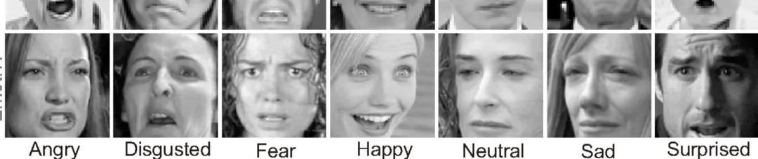
面部表情丰富多样，包含angry(生气), disgust (厌恶), fear(害怕), happy(快乐), neutral (中性), sad(悲伤), surprise(惊奇)等多种表情。

数据结构

该数据集包含了48×48像素的灰度人脸图像。这些人脸已经自动注册，使得人脸在每个图像中大致居中并占据大约相同的空间。任务是根据面部表情中显示的情感将每个人脸分类为七个类别之一（0=愤怒，1=厌恶，2=恐惧，3=快乐，4=悲伤，5=惊讶，6=中性）。

文件：fer2013.csv

emotion	pixels	Usage
0	70 80 82 72 58 58 60 …	Training
0	151 150 147 155 148 …	Training
2	231 212 156 164 174 …	Training

“emotion”列包含一个从0到6（包含0和6）的数字代码，表示图像中存在的情感。”pixels”列包含一个用引号包围的字符串，对于每个图像都有一个。这个字符串的内容是以行为主顺序排列的空格分隔的像素值。

完整版数据集包括已换成表情图片文件集合，一个文件目录标注一组人脸表情图片。

0_Neutral
1_Anger
2_Disgust
3_Fear
4_Happy
5_Sad
6_Surprise

数据集使用许可协议

Database Contents License (DbCL) v1.0 — Open Data Commons: legal tools for open data

三、识别样例

两种使用方法

方法1：使用已构建的模型

如果你不想从头开始训练分类器，你可以直接使用fertestcustom.py，因为仓库中已经有了fer.json（训练好的模型）和fer.h5（参数），这些可以用来预测文件夹中任何测试图像的情绪。你可以根据你的需求修改fertestcustom.py，并用它来预测任何用例中的面部情绪。

方法2：从数据源从零构建模型

数据源：fer2013.csv

运行 preprocessing.py 文件，这将为你生成 fadataX.npy 和 flabels.npy 文件。运行 fertrain.py 文件，这会根据你的处理器和显卡的不同而花费一些时间。这将为你创建 modXtest.npy、modytest.npy、fer.json 和 fer.h5 文件。

安装开发包

参考文章《安装深度学习框架TensorFlow》。

以tensorflow_gpu-2.6.0的安装为例，查表可获知该版本依赖于python3.6-3.9。

conda create -n tensorflow-gpu-2-6-p3-9 python=3.9
conda activate tensorflow-gpu-2-6-p3-9
conda install tensorflow-gpu==2.6

查看已安装的tensorflow版本信息：

conda list tensor
# packages in environment at D:\App-Data\conda3\envs\tensorflow-gpu-2-6-p3-9:
#
# Name                    Version                   Build  Channel
tensorboard               2.6.0                      py_1    anaconda
tensorboard-data-server   0.6.1            py39haa95532_0    anaconda
tensorboard-plugin-wit    1.8.1            py39haa95532_0    anaconda
tensorflow                2.6.0           gpu_py39he88c5ba_0    anaconda
tensorflow-base           2.6.0           gpu_py39hb3da07e_0    anaconda
tensorflow-estimator      2.6.0              pyh7b7c402_0    anaconda
tensorflow-gpu            2.6.0                h17022bd_0    anaconda

同时安装

 conda install numpy==1.20.3
 conda install sklearn pandas opencv-python

1、预处理

这段代码的主要目的是将FER2013数据集预处理成适合深度学习模型训练的格式，并将其保存为NumPy数组文件，以便后续使用。

preprocessing.py

import pandas as pd
import numpy as np
import warnings
warnings.filterwarnings("ignore")

data = pd.read_csv('./data/fer2013/fer2013.csv')

width, height = 48, 48

datapoints = data['pixels'].tolist()

#getting features for training
X = []
for xseq in datapoints:
    xx = [int(xp) for xp in xseq.split(' ')]
    xx = np.asarray(xx).reshape(width, height)
    X.append(xx.astype('float32'))

X = np.asarray(X)
X = np.expand_dims(X, -1)

#getting labels for training
y = pd.get_dummies(data['emotion']).to_numpy()

#storing them using numpy
np.save('./preprocess/fdataX', X)
np.save('./preprocess/flabels', y)

print("Preprocessing Done")
print("Number of Features: "+str(len(X[0])))
print("Number of Labels: "+ str(len(y[0])))
print("Number of examples in dataset:"+str(len(X)))
print("X,y stored in fdataX.npy and flabels.npy respectively")

python preprocessing.py

输出：./preprocess/fdataX.npy 和 ./preprocess/flabels.npy 文件

Preprocessing Done
Number of Features: 48
Number of Labels: 7
Number of examples in dataset:35887
X,y stored in fdataX.npy and flabels.npy respectively

2、训练和执行结果

这段代码是一个典型的深度学习模型的训练过程，主要使用Keras API构建和训练一个卷积神经网络（CNN）。这段代码是一个完整的深度学习模型训练流程，适用于图像分类任务。流程如下：

数据预处理：标准化输入数据。
数据分割：将数据分为训练集、验证集和测试集。
模型构建：构建一个深度CNN模型，包含多个卷积层、批归一化层、池化层和Dropout层。
模型编译：使用Adam优化器和分类交叉熵损失函数。
模型训练：训练模型并使用验证集进行验证。
模型保存：将模型结构和权重保存到文件中，以便后续使用。

源码：fertrain.py

输入：./preprocess/fdataX.npy和./preprocess/flabels.npy

输出：./model/fer.json 和 ./model/fer.h5

import sys, os
import pandas as pd
import numpy as np
from sklearn.model_selection import train_test_split

import tensorflow as tf
from tensorflow.keras.models import Sequential
from tensorflow.keras.layers import Dense, Dropout, Activation, Flatten, Conv2D, MaxPooling2D, BatchNormalization
from tensorflow.keras.losses import CategoricalCrossentropy
from tensorflow.keras.optimizers import Adam
from tensorflow.keras.regularizers import l2
from tensorflow.keras.callbacks import ReduceLROnPlateau, TensorBoard, EarlyStopping, ModelCheckpoint
from tensorflow.keras.models import load_model
from tensorflow.keras.models import model_from_json


num_features = 64
num_labels = 7
batch_size = 64
epochs = 100
width, height = 48, 48

x = np.load('./preprocess/fdataX.npy')
y = np.load('./preprocess/flabels.npy')

x -= np.mean(x, axis=0)
x /= np.std(x, axis=0)

#for xx in range(10):
#    plt.figure(xx)
#    plt.imshow(x[xx].reshape((48, 48)), interpolation='none', cmap='gray')
#plt.show()

#splitting into training, validation and testing data
X_train, X_test, y_train, y_test = train_test_split(x, y, test_size=0.1, random_state=42)
X_train, X_valid, y_train, y_valid = train_test_split(X_train, y_train, test_size=0.1, random_state=41)

#saving the test samples to be used later
np.save('./model/modXtest', X_test)
np.save('./model/modytest', y_test)

#desinging the CNN
model = Sequential()

model.add(Conv2D(num_features, kernel_size=(3, 3), activation='relu', input_shape=(width, height, 1), data_format='channels_last', kernel_regularizer=l2(0.01)))
model.add(Conv2D(num_features, kernel_size=(3, 3), activation='relu', padding='same'))
model.add(BatchNormalization())
model.add(MaxPooling2D(pool_size=(2, 2), strides=(2, 2)))
model.add(Dropout(0.5))

model.add(Conv2D(2*num_features, kernel_size=(3, 3), activation='relu', padding='same'))
model.add(BatchNormalization())
model.add(Conv2D(2*num_features, kernel_size=(3, 3), activation='relu', padding='same'))
model.add(BatchNormalization())
model.add(MaxPooling2D(pool_size=(2, 2), strides=(2, 2)))
model.add(Dropout(0.5))

model.add(Conv2D(2*2*num_features, kernel_size=(3, 3), activation='relu', padding='same'))
model.add(BatchNormalization())
model.add(Conv2D(2*2*num_features, kernel_size=(3, 3), activation='relu', padding='same'))
model.add(BatchNormalization())
model.add(MaxPooling2D(pool_size=(2, 2), strides=(2, 2)))
model.add(Dropout(0.5))

model.add(Conv2D(2*2*2*num_features, kernel_size=(3, 3), activation='relu', padding='same'))
model.add(BatchNormalization())
model.add(Conv2D(2*2*2*num_features, kernel_size=(3, 3), activation='relu', padding='same'))
model.add(BatchNormalization())
model.add(MaxPooling2D(pool_size=(2, 2), strides=(2, 2)))
model.add(Dropout(0.5))

model.add(Flatten())
model.add(Dense(2*2*2*num_features, activation='relu'))
model.add(Dropout(0.4))
model.add(Dense(2*2*num_features, activation='relu'))
model.add(Dropout(0.4))
model.add(Dense(2*num_features, activation='relu'))
model.add(Dropout(0.5))

model.add(Dense(num_labels, activation='softmax'))

#model.summary()

#Compliling the model with adam optimixer and categorical crossentropy loss
# model.compile(loss=CategoricalCrossentropy,
#               optimizer=Adam(lr=0.001, beta_1=0.9, beta_2=0.999, epsilon=1e-7),
#               metrics=['accuracy'])
model.compile(loss=CategoricalCrossentropy(),
              optimizer=Adam(learning_rate=0.001, beta_1=0.9, beta_2=0.999, epsilon=1e-7),
              metrics=['accuracy'])

model.fit(np.array(X_train), np.array(y_train),
          epochs=100,
          batch_size=32,
          validation_split=0.2)  


#saving the  model to be used later
fer_json = model.to_json()
with open("./model/fer.json", "w") as json_file:
    json_file.write(fer_json)
model.save_weights("./model/fer.h5")
print("Saved model to disk")

python fertrain.py

输出：./model/fer.json 和 ./model/fer.h5

726/727 [============================>.] - ETA: 0s - loss: 2.0054 - accuracy: 0.21842024-12-04 15:04:16.066255: W tensorflow/core/common_runtime/bfc_allocator.cc:272] Allocator (GPU_0_bfc) ran out of memory trying to allocate 1.17GiB with freed_by_count=0. The caller indicates that this is not a failure, but may mean that there could be performance gains if more memory were available.
727/727 [==============================] - 167s 148ms/step - loss: 2.0053 - accuracy: 0.2183 - val_loss: 1.8289 - val_accuracy: 0.2401
Epoch 2/100
727/727 [==============================] - 106s 145ms/step - loss: 1.8399 - accuracy: 0.2461 - val_loss: 1.8082 - val_accuracy: 0.2504
Epoch 3/100
727/727 [==============================] - 109s 150ms/step - loss: 1.7840 - accuracy: 0.2691 - val_loss: 1.6917 - val_accuracy: 0.3091
Epoch 4/100
727/727 [==============================] - 114s 156ms/step - loss: 1.6970 - accuracy: 0.3108 - val_loss: 1.6057 - val_accuracy: 0.3493
...

3、识别预测

源码：fertest.py

输入：modXtest.npy、modytest.npy、fer.json 和 fer.h5 文件。

这段代码执行了以下操作：

从文件中加载了一个Keras模型的架构。
加载了与模型架构对应的权重。
打印了一条消息，确认模型已从磁盘加载。
初始化了两个空列表truey和predy，用于存储真实标签和预测标签。
从.npy文件中加载了测试数据x和对应的标签y。
使用加载的模型对测试数据x进行预测，并将预测结果存储在yhat中。
将预测结果和真实标签转换为列表格式。
遍历每个样本，找到预测概率最高的类别索引，并将其添加到predy列表中；同样地，找到真实标签中概率最高的类别索引，并将其添加到truey列表中。
如果预测类别索引与真实类别索引相同，则计数器count加1。
计算并打印测试集上的准确率。
将真实标签和预测标签保存到.npy文件中，以便后续进行混淆矩阵分析等。
打印一条消息，确认预测和真实标签值已保存。

输出将包括以下内容：

“Loaded model from disk”：确认模型已成功从磁盘加载。
“Predicted and true label values saved”：确认预测和真实标签值已保存到文件中。
“Accuracy on test set :XX%”：显示测试集上的准确率，其中XX是一个具体的数字，表示准确率的百分比。

# load json and create model
from __future__ import division

import tensorflow as tf
from tensorflow.keras.models import Sequential
from tensorflow.keras.layers import Dense
from tensorflow.keras.models import model_from_json

import numpy
import os
import numpy as np

json_file = open('./model/fer.json', 'r')
loaded_model_json = json_file.read()
json_file.close()
loaded_model = model_from_json(loaded_model_json)
# load weights into new model
loaded_model.load_weights("./model/fer.h5")
print("Loaded model from disk")

truey=[]
predy=[]
x = np.load('./model/modXtest.npy')
y = np.load('./model/modytest.npy')

yhat= loaded_model.predict(x)
yh = yhat.tolist()
yt = y.tolist()
count = 0

for i in range(len(y)):
    yy = max(yh[i])
    yyt = max(yt[i])
    predy.append(yh[i].index(yy))
    truey.append(yt[i].index(yyt))
    if(yh[i].index(yy)== yt[i].index(yyt)):
        count+=1

acc = (count/len(y))*100

#saving values for confusion matrix and analysis
np.save('truey', truey)
np.save('predy', predy)
print("Predicted and true label values saved")
print("Accuracy on test set :"+str(acc)+"%")

源码开源协议

MIT license

四、获取案例套装